

BLH Experimental Demonstration Research Design
Summer 2019 Demonstration Project: Tomatoes
Objective
Determine differences between growth and condition of tomatoes using Aquatonix treated water vs non-treated water
Summary of Results
Running the Welch t test, a p-value of 0.4205 was calculated; the hypothesis is NOT rejected and there is no statistically significant difference in the two groups. This means, neither the Aquatonix treated tomato fruits or the non-treated tomato fruits weigh more or less, they are statistically identical.
Project
Use of 6 raised beds randomly assigned demonstrate use of Aquatonix to students and growers. Tomatoes will be grown with no differences between treatment and control beds except for the source of water.
BLH Agrees to:
- Provide Aqutonix to the participant free of charge;
- Coordinate delivery of Aqutonix to the participant's designated location;
- Provide a product installation and maintenance manual;
- Provide a $xxxx stipend for a student to oversee the Project including data collection, irrigation system, documentation of growth and harvest, and care of the plants;
- Provide $xxxx for costs associated of piping, tubing, control valves, and gauges required for irrigation system to use the Aqutonix machine;
- Be responsible for the costs of testing water and soil for baseline data; and the costs of testing tissues and fruit during the test plan.
Coalinga CollegeAgree to:
- Use Aqutonix treated water on treatment beds and nontreated water on control beds from the beginning of planting to harvest.
- Maintain cultural and production practices on all treated and control beds
- Provide measurement and images of product growth, yield, and quality throughout the
growing season. This includes but is not limited to:
- Weight of crops that had to be discarded due to pests and diseases
- Individual crop weight and size of control and treated crops (please include image of five pieces of the fruit or vegetable on a scale)
- Sugar content of control and treated crops
Data Gathering Phase:
We decided to harvest on July 18th to get accurate weights and representations without any worry of potential heat damage. We determined it would be efficient if we cut all the tomato plants where the stalk met the dirt. We weighed the whole biomass of the box (that is, all the plants and fruits of a box) together for total biomass, picked all the fruit off of the plants and took the total fruit weight and then randomly sampled the tomato fruits and took ten individual tomato fruit weights. Some of the boxes had about 50-75 tomatoes which we wouldn’t have been able to weigh every single fruit individually in the same day. Industry practice is to take weights for a whole strip of tomatoes, not individual fruits. We also decided to randomly sample some of the tomatoes and take individual fruit weights, so we could see how the actual tomato fruits did in BLH versus Nontreated boxes. This is also an industry practice. When a truck full of tomatoes pulls up to a processing station, a sieve lowers down into the truck and pulls a random sample of the tomatoes to determine the overall characteristics of the tomato fruit in that truck. We implored the same practice, randomly sampling ten fruits from the whole box weight. This means we recorded a weight for the total biomass of a box (greens + fruits), total tomato fruit from a box, and ten randomly sampled tomato fruits from the aggregated overall tomato weight box.
Detailed Results:
Descriptive Stats:
All of the data gathered in the field was recorded by me with pen and paper, and was double checked and verified each time. I entered all these weights into excel sheets so I could pull them into my statistical software package I use for analysis (R software). Descriptive stats are important to explore insights in data, look for trends/ differences, and have some comparability to start with. I will not list a few tables of descriptive stats on the tomatoes. Before we begin, I will give an image on how the boxes are being referenced this time. Where Box 1 and Box 4 are the north most boxes and Box 3 and Box 6 are the most south (imagine you are starting in front of the boxes looking towards the field). I will also include photos to make this point more clear.
| Box 3 | Box 6 |
| Box2 | Box 5 |
| Box 1 | Box 4 |
Weights of Boxes: Biomass, Total Fruit and Greens
| Weight of Biomass (g) | Weight of Tomatoes (g) | Weight of Greens (g) | Box Number | Treatment |
| 6441.01 | 2449.40 | 3991.61 | 1 | 0 |
| 7348.19 | 1905.09 | 5443.10 | 2 | 0 |
| 7711.06 | 1814.37 | 5896.70 | 3 | 1 |
| 6168.85 | 1542.21 | 4626.64 | 4 | 1 |
| 6713.16 | 1995.80 | 4717.36 | 5 | 1 |
| 5715.26 | 1632.93 | 4082.33 | 6 | 0 |
Where treatment is a binary variable for BLH =1, Nontreated = 0.
To reiterate here, the biomass weight is the green of the plant + fruits on the plants. We also have the weight for ALL tomatoes from that box. Initially inspecting this table, we can see that for overall weights, The BLH had the highest biomass weight. When you look at the weight of the tomatoes, the nontreated box had the most/heaviest tomatoes in Box 1 but BLH had the second highest in Box 5. The BLH boxes had really heavy greens (plants with no fruits), and had the 1st , 3rd and 4th place in terms of weights of the greens. On initially inspections, it appears BLH water heavily increases the greens of the plant but that may not translate/transfer into the fruits of the plant or may take longer than the nontreated water does to move into the fruit. It is hard to determine that here, and would probably be another person’s expertise. Now let’s look at the randomly sampled fruits’ descriptive stats.
Tomato fruit Weights:
| *In grams | Box 1 | Box 2 | Box 3 | Box 4 | Box 5 | Box 6 |
| Min | 21 | 17 | 12 | 13 | 13 | 15 |
| Median | 26.5 | 26 | 25 | 25.5 | 21 | 24.5 |
| Mean | 27.4 | 26.7 | 22.6 | 25.1 | 24.8 | 22.8 |
| Max | 40 | 45 | 30 | 31 | 42 | 28 |
| BLH Weights (grams) | |||
| Min | Median | Mean | Max |
| 12 | 24.5 | 24.17 | 42 |
| Nontreated Weights (grams) | |||
| Min | Median | Mean | Max |
| 15 | 25.5 | 25.63 | 45 |
As discussed above, we randomly sampled ten fruits from the bin we took the total fruit weight from. This means we got sixty weighted values for tomato fruits. I have put them together here in a table by Boxes and then by BLH vs Nontreated tomato fruits. The first table is comparing the ten fruits sampled in each box, while the second and third tables are looking at all thirty BLH tomatoes versus all thirty Nontreated tomatoes. Again to remind, Boxes 3, 4 and 5 are BLH while Boxes 1, 2 and 6 are Nontreated. It appears that Box 3 had the smallest fruit ( and was really close to Boxes 4 and 5) while Box 2 had the largest fruit of the trial with Box 5 really close by. The BLH boxes had a lot of tomatoes on them that were smaller, and so it was more probable that a smaller tomato would be chosen at random. You will see this in the photos attached of the Box 3 tomatoes. When we look at the Median and Means of the boxes we see they are pretty close in values with Box 6 have the largest variance in the Median and Mean values. This means that there were more smaller fruits that got sampled which pulled the mean down, while the opposite is true in Box 5 where mostly larger fruits were sampled which pulled the Mean up.
When we look at the BLH vs Nontreated all together (30 fruits vs 30 fruits) we see they are relatively close in size. We see the nontreated fruits have a higher min and max value, with their median and mean values relatively close which means no outlier is pulling the Mean value up or down. The same can be said for the BLH values as they are relative close and may have more smaller fruits overall than the nontreated boxes did.
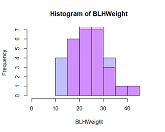
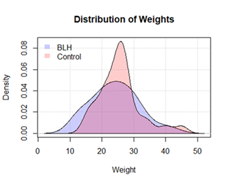
We can visually see this too if we look at the distributions of the fruits. In the first histogram, blue is BLH while red is Nontreated fruits. Any purple region is overlap between the two groups and we can see there is a lot of overlap between the two with quite a few BLH weights in the very first bin (smaller fruits). We can see this better if we turn the histogram into a density plot. Now we can better visually the distribution of the two groups. We see the control group has a spike in the 20-30 range while BLH has a smoother trend in the weights. We can also better visualize the overlap between the two groups.
This does not mean there is any bad values or anything worse off by the BLH water here on visual inspection. We need to statistically test if these weights are statistically significantly different from each other, or if these distributions are the same meaning no effect one way or the other. To do this, we need to process the data into a statistical software and begin some testing.
Statistical Testing:
When we test a treatment versus a control we expect the two groups to not overlap. Graphics, however, are not the official way we test to see if two groups are different. To do this, we can utilize the Welch two Sample t-test to test whether or not two groups are statistically different from each other. The test itself is looking to see whether the true difference in the means is equal to zero, written in the statistical notation
H0 (Null hypothesis) = True difference in means equals zero
HA (Alternative Hypothesis) = True difference in means is not equal to zero
If we reject the hypothesis, then we are saying a difference is present. However, if we fail to reject the null hypothesis that means there is no difference in the means between the groups.
We will make the decision on rejecting/failing to reject based on the p-value from the Welch test. If the p-value is above the significance level (here we assume a 95% significance level, as that is common practice. Without lecturing completely on statistics, we want to compare the p-value to our set alpha level which is assumed to be 0.05 for a 95% significance. If p-value is less than 0.05 we will reject the null (difference present) or if it is greater than 0.05 we will fail to reject (no difference present)). I will begin by comparing the actual tomato fruits and then will expand out to tests for differences in other places (location, biomass, greens, total fruit).
Results:
Running the Welch t test, I found a p-value of 0.4205. This means I fail to reject the hypothesis and there is no statistically significant difference in the two groups. This means neither the BLH tomato fruits or the Nontreated tomato fruits weigh more or less, they are statistically identical.
When I tested the North end (Box 1, Box 4) versus South end (Box 3, Box 6) tomato fruits I found a p-value of 0.04962 which means I reject the null hypothesis (even though it is very very close to the cutoff point), meaning there is a statistically significant difference present in this comparison. This means there may be a spatial component in effect here, and you can see this if you look at the deceptive stats on the boxes. However, if you try to test this further and compare North vs South treatment and control boxes, you do not pick up any statistically significant difference in individual boxes, only when you look at the North and South end together. I would call this a relative weak difference.
Of all the other tests I mentioned above (biomass, greens, total fruit) I fail to reject all of these for any statistically significant difference in the groups (p-value of .6083,.4093,.4941 respectively).